Quantum Mechanics has been an all-time favorite topic for all science nerd, however, it’s truly a tedious job to understand the quantum phenomena and even more tedious when it comes to experimenting these effects (To know the three eras of quantum mechanics, check out my post ‘Journey through the quantum mechanics‘). One such experiment is making an economically viable and efficient Quantum Computer (to understand its working, visit ‘how quantum computers work? (beginners edition)‘). Decoherence is one of the biggest challenges when it comes to quantum computers, since, a tiny noise can affect the arrangement of the atoms and can break the quantum phenomena. 

There are many processes used to make a quantum computer like the optic trap, quantum dot (semiconductor), superconducting qubits and ion trap. However, all these methods need to maintain the microscopic scale and handling objects at such scales is extremely difficult. Using macroscopic techniques that we use in our classical computers is not possible in quantum computers, since, quantum effects cannot be seen in a macroscopic world. However, there is an exception to this rule. 

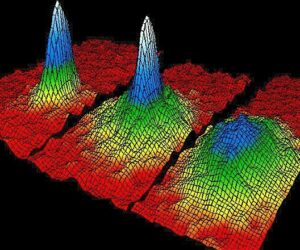
Bose-Einstein Condensate is one exception that shows microscopic phenomena at a macroscopic scale. For example, in a Bose-Einstein Condensate, all the bosons in the system occupy the ground state of the trap.  The state of the system then obeys a macroscopic wave-function obeying the Gross-Pitaevskii equation, which has a similar mathematical form as the Schrodinger equation.  This similar structure causes the macroscopic wave-function to obey all the same properties as microscopic quantum particles such as superposition and tunneling, but on a macroscopic scale.

The Bose-Einstein Condensate was first proposed by S. N. Bose and was further developed along with Albert Einstein. The theory ‘Bose-Einstein Statistics’ predicts that at the absolute temperature the bosons will adopt the same energy state. Bosons are the particles with an integer spin and they do not follow Pauli’s exclusion principle, thus, they behave differently than fermions at extremely low temperatures. 

In 1900, Planck proposed Planck’s law which describes the spectral density of electromagnetic radiation emitted by a black body in thermal equilibrium at a given temperature T. However, experimental data didn’t fit the theoretical data at a microscopic scale. 

S. N. Bose studied the first factor in Planck’s law and figured out the probability of finding particles in various states in phase space, where each state is a little patch having volume h³, and the position and momentum of the particles are not kept particularly separate but are considered as one variable. Phase space refers to the plotting of both a particle’s momentum and position on a two-dimensional graph. It also refers to the tracking of N particles in a 2N dimensional space. Bose proposed that the total number of cells must be regarded as the number of arguments of a single quantum in the given volume. If A^s denotes the number of cells in the frequency range dv in unit volume, one can calculate the number of possible ways to arrange N^s quanta in these cells. Cells here are quantized states of light and these cells with a given number of quanta are indistinguishable. 

We can derive a probabilistic equation for A^s and get (4πv²dv) ÷ (c³), however, this is not the correct equation. To get an accurate equation for A^s we have to multiply by a factor of 2. This factor of two indicates the internal degree of freedom of the electromagnetic field. This is which Bose identified with the helicity of its quanta i.e. the components of its intrinsic spin parallel and anti-parallel to its direction of motion. Therefore,

A^s = (8πv²dv) ÷ (c³)

Let us place a single quantum of type s randomly in one of the cells and then a second identical quantum, also randomly, in one of the cells, then a third one and so on. This way one will get one possible arrangement of N^s identical quanta in the A^s cells i.e. one complexion. If this procedure is repeated a sufficiently large number of times, all possible complexions will be obtained. Let p^s₀ be the number of empty cells, p^s₁ the number of cells in 1 quantum, p^s₂ the number of cells in 2 quanta, etc. obtained in this way. It is clear from this that the phase cells are distinguished only by their occupation numbers. Hence, cells with a given number of quanta are indistinguishable. In other words, the different arrangements of the quanta in cells with a given number of quanta are indistinguishable. Since all complexions are equally probable, the probability of a state of type s quanta can be given as:

W^s = A^s! ÷ (p^s₀!p^s₁!p^s₂!…p^s_r!)

Therefore, the macroscopically defined probability of a state defined by all types of quanta can be given as:

W = Π_s W^s = Π_s  [A^s! ÷ (p^s₀!p^s₁!p­^s₂!…p^s_r!)]

If one maximizes the entropy S = -klogW subject to the constraints that the total energy is the sum of the energies of all the quanta, E = Σ_s N^s h v^s and the total number of quanta is the sum of the numbers of quanta in all the states, N^s = Σ_rrp^s_r, one obtains in the limit of large numbers p^s_r the statistical Planck factor (e^hv/kT – 1)^-1

We thus see that the indistinguishability of photons was not an ad hoc assumption in Bose derivation of Planck’s law. It followed from the quantization of the electromagnetic phase space. Bose’s derivation shows clearly that it is not the photons but the quantized states of an electromagnetic field that are the independent degrees of freedom of the system, and that states with the same number of identical photons are indistinguishable. It is the critical clue to the Fock space formulation of the quantum electrodynamics that followed later. 

One important point to mention is that Planck’s law can be derived in two ways; one with indistinguishability of quantum states radiation by quantizing the electromagnetic field as Bose did and use the distribution and other by retaining the classical wave character of the electromagnetic field, postulating the indistinguishability of quanta and use the Debye distribution.

After deriving Planck’s law by Bose, Einstein extended Bose’s methods to develop the quantum theory of ideal gas. He used the Debye form of the distribution with the additional assumption of conservation of the number of atoms. Since the gas atoms were indistinguishable by hypothesis, their tracks under mutual exchange became unobservable, leading to their wave nature. 

Einstein connected these matter waves with de Broglie waves with wavelength λ = h/p where the momentum p = √(2mkT). Hence, λ α 1/√(T), and the wavelength was predicted to increase as the temperature of the gas was lowered. Consequently, he showed that the waves of the individual atoms would start to overlap more and more as the temperature was lowered, so that below a very critical temperature, the waves would overlap so much that the atoms would lose their identities completely and condense into the lowest quantum state, behaving like a giant atom with wave character. Such a state came to be known as the Bose-Einstein Condensate (BEC).

In this post, I have used mathematical formulation which otherwise I don’t use much. I would like to know your response down below. Based on your comments I will make my future posts 🙂